Skip to main content

Measuring distance between texts

Compare string distance with vector distance

Learn how string and vector distances answer different similarity questions, and why raw-count Euclidean distance depends on document length.

Matching a mistyped name requires a different comparison from matching the vocabulary of two paragraphs. Both tasks measure similarity, but they compare different features.

A distance measure expresses a comparison as a number. A smaller distance indicates greater similarity under that measure. Choose a distance measure that matches the question.

TipWhat you will learn

This lesson shows how to:

• compare edit distance and Jaro-Winkler distance for names
• build paragraph vectors from word counts
• compare cosine, Euclidean, and Jaccard distance
• measure how strongly a distance reflects text length
• explain why the same data can give different rankings.

Compare strings directly

String distance compares characters. Levenshtein distance counts edits: insertions, deletions, and substitutions. Jaro-Winkler distance assigns greater similarity to strings with a shared prefix, or beginning. This adjustment often helps with names.

library(dplyr)
library(tibble)
library(stringr)
library(stringdist)
library(quanteda)
library(Matrix)
library(ggplot2)

source("R/permutation-null.R")

within_tolerance <- function(observed, expected, tolerance = 1e-3) {
  abs(observed - expected) < tolerance
}

name_matches <- tibble(
  recorded = c("Jonson", "Jonson", "Martha", "Martha", "Stevenson", "Stevenson"),
  candidate = c("Johnson", "Jansen", "Marta", "Marsha", "Stephenson", "Steven")
) |>
  mutate(
    levenshtein = stringdist(recorded, candidate, method = "lv"),
    jaro_winkler = stringdist(recorded, candidate, method = "jw", p = 0.1),
    levenshtein_rank = rank(levenshtein, ties.method = "first"),
    jaro_winkler_rank = rank(jaro_winkler, ties.method = "first")
  )

stevenson_rows <- name_matches |>
  filter(recorded == "Stevenson")

Two string distances rank the same candidate names differently

Recorded	Candidate	Levenshtein	Jaro-Winkler	Levenshtein rank	Jaro-Winkler rank
Jonson	Johnson	1	0.0381	1	2
Jonson	Jansen	2	0.2000	4	6
Martha	Marta	1	0.0333	2	1
Martha	Marsha	1	0.0778	3	5
Stevenson	Stephenson	2	0.0726	5	4
Stevenson	Steven	3	0.0667	6	3

For Stevenson, Levenshtein selects Stephenson because the match requires fewer edits. Jaro-Winkler selects Steven because of the shared prefix. Choose the distance measure that reflects the spelling errors relevant to the project.

Build paragraph vectors

A vector is a row of numbers. In a document-feature matrix, each row is a paragraph and each column is a word feature. The entry says how many times that word appears in that paragraph.

source("R/inaugural-corpus.R")

paragraphs <- inaugural_paragraphs()

paragraph_tokens <- tokens(
  paragraphs$paragraph,
  remove_punct = TRUE,
  remove_numbers = TRUE
) |>
  tokens_tolower()

paragraph_dfm <- dfm(paragraph_tokens)
docnames(paragraph_dfm) <- paragraphs$paragraph_id

count_matrix <- as(paragraph_dfm, "dgCMatrix")
token_lengths <- Matrix::rowSums(count_matrix)
squared_lengths <- Matrix::rowSums(count_matrix^2)
dot_products <- as.matrix(Matrix::tcrossprod(count_matrix))

euclidean_squared <- outer(squared_lengths, squared_lengths, "+") - 2 * dot_products
euclidean_squared[euclidean_squared < 0 & euclidean_squared > -1e-8] <- 0
euclidean_distance <- sqrt(euclidean_squared)

vector_norms <- sqrt(squared_lengths)
cosine_similarity <- dot_products / outer(vector_norms, vector_norms)
cosine_distance <- 1 - cosine_similarity

binary_matrix <- Matrix::drop0(count_matrix)
binary_matrix@x <- rep(1, length(binary_matrix@x))
feature_counts <- Matrix::rowSums(binary_matrix)
intersections <- as.matrix(Matrix::tcrossprod(binary_matrix))
unions <- outer(feature_counts, feature_counts, "+") - intersections
jaccard_distance <- 1 - intersections / unions

pair_index <- which(upper.tri(euclidean_distance), arr.ind = TRUE)
pair_distances <- tibble(
  first = pair_index[, 1],
  second = pair_index[, 2],
  length_difference = abs(token_lengths[first] - token_lengths[second]),
  euclidean = euclidean_distance[pair_index],
  cosine = cosine_distance[pair_index],
  jaccard = jaccard_distance[pair_index],
  first_speech = paragraphs$speech_id[first],
  second_speech = paragraphs$speech_id[second]
)

Paragraph vectors built from the inaugural-address corpus

Item	Value
Paragraphs	1377
Speeches	60
People	40
Features	9327
Paragraph pairs	947376

The matrix has 1,377 paragraph rows and 9,327 word columns. Each paragraph becomes a point in a high-dimensional space.

Compare three vector distances

Euclidean distance measures straight-line distance between count vectors. Cosine distance compares direction. Multiplying every element of a paragraph vector by the same positive constant leaves its direction unchanged. Jaccard distance uses word presence and ignores repeated counts.

length_correlations <- pair_distances |>
  summarise(
    `Euclidean distance` = cor(euclidean, length_difference),
    `Cosine distance` = cor(cosine, length_difference),
    `Jaccard distance` = cor(jaccard, length_difference)
  ) |>
  tidyr::pivot_longer(
    everything(),
    names_to = "distance",
    values_to = "correlation_with_length_difference"
  )

same_speech_examples <- pair_distances |>
  mutate(
    first_paragraph = paragraphs$paragraph_id[first],
    second_paragraph = paragraphs$paragraph_id[second],
    first_length = as.integer(token_lengths[first]),
    second_length = as.integer(token_lengths[second])
  ) |>
  filter(first_speech == second_speech) |>
  arrange(desc(length_difference), euclidean) |>
  slice_head(n = 3) |>
  transmute(
    first_paragraph,
    second_paragraph,
    speech = first_speech,
    first_length,
    second_length,
    length_difference = as.integer(length_difference),
    euclidean = round(euclidean, 2),
    cosine = round(cosine, 3),
    jaccard = round(jaccard, 3)
  )

Raw-count distance compared with paragraph length difference

Distance	Correlation with length difference
Euclidean distance	0.951
Cosine distance	-0.268
Jaccard distance	0.275

Long and short paragraphs from the same speech can be far apart under Euclidean distance

First paragraph	Second paragraph	Speech	First length	Second length	Length difference	Euclidean	Cosine	Jaccard
1841-Harrison-p10	1841-Harrison-p22	1841-Harrison	984	69	915	147.46	0.330	0.936
1841-Harrison-p10	1841-Harrison-p25	1841-Harrison	984	80	904	145.87	0.304	0.942
1841-Harrison-p10	1841-Harrison-p11	1841-Harrison	984	94	890	142.01	0.229	0.924

The Euclidean correlation with length difference is 0.951, indicating that raw-count distance mostly measures paragraph size. The cosine correlation is negative, -0.268, because longer paragraphs share many ordinary words with other long paragraphs. In this corpus, nineteenth-century paragraphs are longer than later paragraphs. A method sensitive to length can therefore reproduce the era pattern seen in the corpus lessons.

same_speech_observed <- pair_distances |>
  filter(first_speech == second_speech) |>
  summarise(mean_cosine_distance = mean(cosine)) |>
  pull(mean_cosine_distance)

speech_labels <- paragraphs$speech_id
same_speech_null <- permutation_null(
  observed = same_speech_observed,
  replicate_fn = function() {
    shuffled_labels <- sample(speech_labels)
    pair_distances |>
      filter(shuffled_labels[first] == shuffled_labels[second]) |>
      summarise(mean_cosine_distance = mean(cosine)) |>
      pull(mean_cosine_distance)
  },
  replicates = 1000L,
  seed = 5902L,
  alternative = "less"
)

Same-speech paragraph cosine distance compared with shuffled speech labels

Observed	Null mean	Null 5th pct	Null 95th pct	p-value	Replicates	Alternative
0.569	0.577	0.573	0.581	0.003	1000	less

A distance formula will calculate values for any paragraphs it receives. The permutation check compares same-speech paragraph distances with distances after randomly rearranging speech labels. Paragraphs from the same speech are closer under cosine distance. However, length still dominates raw-count Euclidean distance.

source("R/lesson-figures.R")

set.seed(5901)
plot_pairs <- pair_distances |>
  slice_sample(n = 3000) |>
  tidyr::pivot_longer(
    c(euclidean, cosine, jaccard),
    names_to = "distance",
    values_to = "value"
  ) |>
  mutate(
    distance = factor(
      distance,
      levels = c("euclidean", "cosine", "jaccard"),
      labels = c("Euclidean", "Cosine", "Jaccard")
    )
  )

ggplot(plot_pairs, aes(x = length_difference, y = value)) +
  geom_point(alpha = 0.15, size = 0.7, colour = lesson_colours[["accent"]]) +
  facet_wrap(vars(distance), scales = "free_y") +
  labs(
    title = "Raw Euclidean distance mostly reflects length",
    subtitle = "3,000 randomly selected paragraph pairs. Each panel has its own vertical scale.",
    x = "Difference in paragraph length, in tokens",
    y = "Distance"
  ) +
  theme_lesson(grid = "both")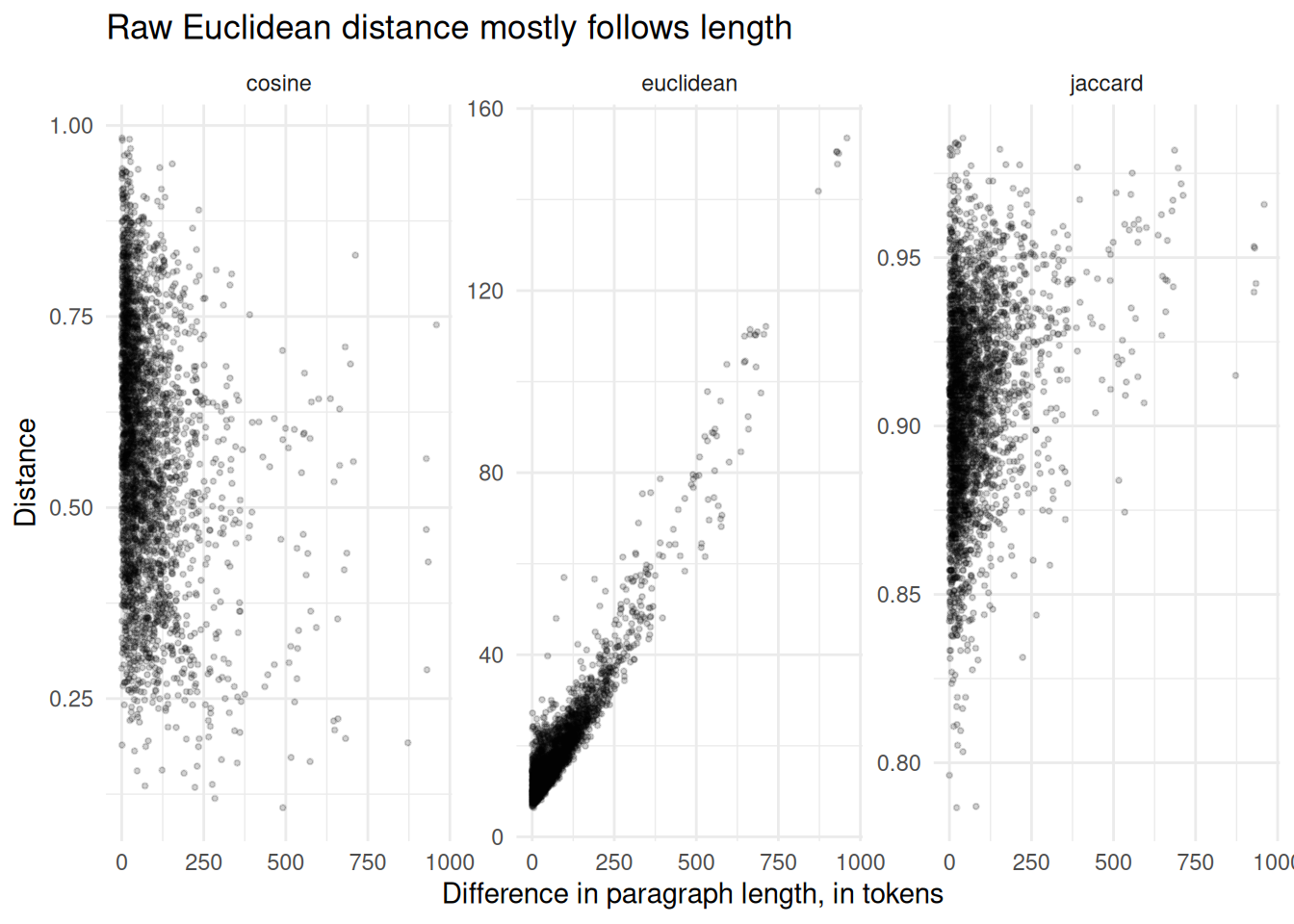

Figure 1: Length difference and distance for a deterministic sample of paragraph pairs.

The plot shows the relationship between length difference and distance. A long paragraph and a short paragraph can have a large raw-count Euclidean distance even when both come from the same speech.

What to remember

• String distance compares character sequences.
• Vector distance compares numeric representations of text.
• Levenshtein and Jaro-Winkler can rank the same name candidates differently.
• On these paragraph counts, Euclidean distance correlates 0.951 with length difference.
• Cosine distance compares direction, which reduces the length problem for raw counts.

Sources

• stringdist package reference
• quanteda tokens documentation
• United States copyright guidance for government works